
(short answer: yes!)
Anyone who develops software that interacts with a database knows (read: should know) how to read a query execution plan, given by “EXPLAIN PLAN”, and how to avoid at least the most common problems like a full table scan.
It is obvious that a plan can change if the database changes. For example if we add an index that is relevant to our query, it will be used to make our query faster. And this will be reflected in the new plan.
Likewise if the query changes. If instead of
SELECT * FROM mytable WHERE somevalue > 5
the query changes to
SELECT * FROM mytable WHERE somevalue IN
  (SELECT someid FROM anothertable)
the plan will of course change.
So during a database performance tuning seminar at work, we came to the following question: can the execution plan change if we just change the filter value? Like, if instead of
SELECT * FROM mytable WHERE somevalue > 5
the query changes to
SELECT * FROM mytable WHERE somevalue > 10
It’s not obvious why it should. The columns used, both in the SELECT and the WHERE clause, do not change. So if a human would look at these two queries, they would select the same way of executing them (e.g. using an index on somevalue if one is available).
But databases have a knowledge we don’t have. They have statistics.
Let’s do an example. We’ll use Microsoft SQL server here. The edition doesn’t really matter, you can use Express for example. But the idea, and the results, are the same for Oracle or any other major RDBMS.
First off, let’s create a database. Open Management Studio and paste the following (changing the paths as needed):
CREATE DATABASE [PLANTEST]
CONTAINMENT = NONE
ON  PRIMARY
( NAME = N'PLANTEST',
FILENAME = N'C:\DATA\PLANTEST.mdf' ,
SIZE = 180MB , FILEGROWTH = 10% )
LOG ON
( NAME = N'PLANTEST_log',
FILENAME = N'C:\DATA\PLANTEST_log.ldf' ,
SIZE = 20MB , FILEGROWTH = 10%)
GO
Note that, by default, I’ve allocated a lot of space, 180MB. There’s a reason for that; We know that we’ll pump in a lot of data, and we want to avoid the delay of the db files growing.
Now let’s create a table to work on:
USE PLANTEST
GO
CREATE TABLE dbo.TESTWORKLOAD
( testid int NOT NULL IDENTITY(1,1),
testname char(10) NULL,
testdata nvarchar(36) NULL )
ON [PRIMARY]
GO
And let’s fill it (this can take some time, say around 5-10 minutes):
DECLARE @cnt1 INT = 0;
DECLARE @cnt2 INT = 0;

WHILE @cnt1 < 20
BEGIN
	SET @cnt2 = 0;
	WHILE @cnt2 < 100000
	BEGIN
	   insert into TESTWORKLOAD (testname, testdata)
             values ('COMMON0001', CONVERT(char(36), NEWID()));
	   SET @cnt2 = @cnt2 + 1;
	END;
	insert into TESTWORKLOAD (testname, testdata)
          values ('SPARSE0002', CONVERT(char(36), NEWID()));
	SET @cnt1 = @cnt1 + 1;
END;
GO
What I did here is, basically, I filled the table with 2 million (20 * 100000) plus 20 rows. Almost all of them (2 million) in the testname field, have the value “COMMON0001”. But a few, only 20, have a different value, “SPARSE0002”.
Essentially the table is our proverbial haystack. The “COMMON0001” rows are the hay, and the “SPARSE0002” rows are the needles 🙂
Let’s examine how the database will execute these two queries:
SELECT * FROM TESTWORKLOAD WHERE testname = 'COMMON0001';
SELECT * FROM TESTWORKLOAD WHERE testname = 'SPARSE0002';
Select both of them and, in management studio, press Control+L or the “Display estimated execution plan” button. What you will see is this:
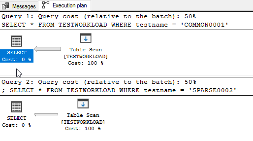
What you see here is that both queries will do a full table scan. That means that the database will go and grab every single row from the table, look at the rows one by one, and give us only the ones who match (the ones with COMMON0001 or SPARSE0002, respectively).
That’s ok when you don’t have a lot of rows (say, up to 5 or 10 thousand), but it’s terribly slow when you have a lot (like our 2 million).
So let’s create an index for that:
CREATE NONCLUSTERED INDEX [IX_testname] ON [dbo].[TESTWORKLOAD]
(
	[testname] ASC
)
GO
And here’s where you watch the magic happen. Select the same queries as above and press Control+L (or the “Display estimated execution plan” button) again. Voila:

What you see here is that, even though the only difference between the two queries is the filter value, the execution plan changes.
Why does this happen? And how?
Well, here’s where statistics are handy. On the Object Explorer of management studio, expand (the “+”) our database and table, and then the “Statistics” folder.

You can see the statistic for our index, IX_testname. If you open it (double click and then go to “details”) you see the following:
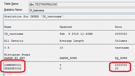
So (I’m simplifying a bit here, but not a lot) the database knows how many rows have the value “COMMON0001” (2 million) and how many the value “SPARSE0002” (just 20).
Knowing this, it concludes (that’s the job of the query optimizer) that the best way to execute the 2 queries is different:
The first one (WHERE testname = ‘COMMON0001’) will return almost all the rows of the table. Knowing this, the optimizer decides that it’s faster to just get everything (aka Full Table Scan) and filter out the very few rows we don’t need.
For the second one (WHERE testname = ‘SPARSE0002’), things are different. The optimizer knows that it’s looking only for a few rows, and it’s smartly using the index to find them as fast as possible.
In plain English, if you want the hay out of a haystack, you just get the whole stack. But if you’re looking for the needles, you go find them one by one.
